Pig

A data flow language and execution environment for exploring very large datasets.Pig runs on HDFS and MapReduce clusters.
Pig has two execution types or modes: local mode and MapReduce mode.

Local Mode: To run the scripts in local mode, no Hadoop or HDFS installation is required. All files are installed and run from your local host and file system.
Mapreduce Mode: To run the scripts in mapreduce mode, you need access to a Hadoop cluster and HDFS installation.

Local mode
In local mode, Pig runs in a single JVM and accesses the local filesystem. This mode is suitable only for small datasets and when trying out Pig. The execution type is set using the -x or -exectype option. To run in local mode, set the option to local: % pig -x local

MapReduce mode
To run the scripts in MapReduce mode

Running the Pig Scripts in Local Mode
To run the Pig scripts in local mode, do the following:
1. Move to the pigtmp directory.
2. Execute the following command using script1-local.pig (or script2-local.pig).
$ pig -x local script1-local.pig
The output may contain a few Hadoop warnings which can be ignored:
3. A directory named script1-local-results.txt (or script2-local-results.txt) is created. This directory contains the results file, part-r-0000.

Running the Pig Scripts in Mapreduce Mode
To run the Pig scripts in mapreduce mode, do the following:
1. Move to the pigtmp directory.
2. Copy the excite.log.bz2 file from the pigtmp directory to the HDFS directory.
$ hadoop fs –copyFromLocal excite.log.bz2 .

What is Flume

Flume is a distributed, reliable, and available service for efficiently collecting, aggregating, and moving large amounts of log data soon after the data is produced.. It has a simple and flexible architecture based on streaming data flows.It uses a simple extensible data model that allows for online analytic applications.
The primary use case for Flume is as a logging system that gathers a set of log files on every machine in a cluster and aggregates them to a centralized persistent store such as the Hadoop Distributed File System (HDFS).

Flume can only write data through a flow at the rate that the final destinations can accept. Although Flume is able to buffer data inside a flow to smooth out high-volume bursts, the output rate needs to be equal on average to the input rate to avoid log jams. Thus, writing to a scalable storage tier is advisable. For example, HDFS has been shown to scale to thousands of machines and can handle many petabytes of data.
HDFS is the primary output destination, events can be sent to local files, or to monitoring and alerting applications such as Ganglia or communication channels such as IRC.HDFS, MapReduce, and Hive, Flume provides simple mechanisms for output file management and output format management. Data gathered by Flume can be processed easily with Hadoop and Hive.

Flume Architecture

Flume’s architecture is simple, robust, and flexible. The main abstraction in Flume is a stream-oriented data flow. A data flow describes the way a single stream of data is transferred and processed from its point of generation to its eventual destination.Data flows are composed of logical nodes that can transform or aggregate the events they receive.Controlling all this is the Flume Master.
Flume that collects log data from a set of application servers. The deployment consists of a number of logical nodes, arranged into three tiers. The first tier is the agent tier. Agent nodes are typically installed on the machines that generate the logs and are your data’s initial point of contact with Flume. They forward data to the next tier of collector nodes, which aggregate the separate data flows and forward them to the final storage tier.

For example, the agents could be machines listening for syslog data or monitoring the logs of a service such as a web server or the Hadoop JobTracker. The agents produce streams of data that are sent to the collectors; the collectors then aggregate the streams into larger streams which can be written efficiently to a storage tier such as HDFS.
Logical nodes are a very flexible abstraction. Every logical node has just two components - a source and a sink. The source tells a logical node where to collect data, and the sink tells it where to send the data. The only difference between two logical nodes is how the source and sink are configured.

Logical and Physical Nodes
One physical node per machine. Physical nodes act as containers for logical nodes, which are wired together to form data flows. Each physical node can play host to many logical nodes, and takes care of arbitrating the assignment of machine resources between them. So, although the agents and the collectors in the preceding example are logically separate processes, they could be running on the same physical node. Flume gives users the flexibility to specify where the computation and data transfer are done.
Flume is designed with four key goals
Reliability:-
Reliability, the ability to continue delivering events in the face of failures without losing data.Flume can guarantee that all data received by an agent node will eventually make it to the collector at the end of its flow as long as the agent node keeps running. That is, data can be reliably delivered to its eventual destination.There are three supported reliability levels:
1)End-to-end :-reliability level guarantees that once Flume accepts an event.The first thing the agent does in this setting is write the event to disk in a 'write-ahead log' (WAL) so that, if the agent crashes and restarts, knowledge of the event is not lost.After the event has successfully made its way to the end of its flow, an acknowledgment is sent back to the originating agent so that it knows it no longer needs to store the event on disk.
2)Store on failure  :-reliability level causes nodes to only require an acknowledgement from the node one hop downstream. If the sending node detects a failure, it will store data on its local disk until the downstream node is repaired, or an alternate downstream destination can be selected. While this is effective, data can be lost if a compound or silent failure occurs.
3)Best effort :-reliability level sends data to the next hop with no attempts to confirm or retry delivery. If nodes fail, any data that they were in the process of transmitting or receiving can be lost. This is the weakest reliability level, but also the most lightweight.

Scalability :-Scalability is the ability to increase system performance linearly - or better - by adding more resources to the system.When load increases, it is simple to add more resources to the system in the form of more machines to handle the increased load.

Manageability :-Manageability is the ability to control data flows, monitor nodes, modify settings, and control outputs of a large system.The Flume Master is the point where global state such as the data flows can be managed. Via the Flume Master, users can monitor flows and reconfigure them on the fly. The Flume Master has the information required to automatically respond to system changes such as load imbalances, partial failures, or newly provisioned hardware.

Extensibility :-Extensibility is the ability to add new functionality to a system. For example, you can extend Flume by adding connectors to existing storage layers or data platforms. Some general sources include files from the file system, syslog and syslog-ng emulation, or the standard output of a process.

Flume Daemons

Flume Daemons are Flume Master and Flume Node

The Flume Master is the central management point and controls the data flows of the nodes. It is the single logical entity that holds global state data and controls the Flume node data flows and monitors Flume nodes.The nodes periodically contact the Master to transmit a heartbeat and to get their data flow configuration.Flume system is working, you must start a single Flume Master and some Flume nodes that interact with the Master.

The Master can be manually started by executing the following command:
$ flume master
After the Master is started, you can access it by pointing a web browser to http://localhost:35871/. This web page displays the status of all Flume nodes that have contacted the Master, and shows each node’s currently assigned configuration. When you start this up without Flume nodes running, the status and configuration tables will be empty.
The web page contains four tables the Node status table, the Node configuration table, the Physical/Logical Node mapping table, and a Command history table.

The Flume NodeTo start a Flume node, invoke the following command
$ flume node_nowatch

On the master, a node can be in one of several states

HELLO : A new node instance initially contacted the master.
IDLE : A node has completed its configuration or has no configuration.
CONFIGURING: A node has received a configuration and is activating the configuration.
ACTIVE: A node is actively pulling data from the source and pushing data into the sink.
LOST: A node has not contacted the master for an extended period of time (default is after 10x the expected heartbeat period 50s by default)
DECOMMISSIONED: A node has been purposely decommissioned from a master.
ERROR: A node has stopped in an error state.

Flume Commands

$ flume dump console

Reading from a text file, text
$ flume dump 'text("/etc/services")'

Tailing a file name
$ flume dump 'tail("testfile")'

create and write data to the file:
$ echo Hello world! >> testfile

delete the file
$ rm testfile

multiple files by file name
$ flume dump 'multitail("test1", "test2")'

send it data coming from the two different files
$ echo Hello world test1! >> test1
$ echo Hello world test2! >> test2

Newlines are excluded from the events.
tail("file", delim="\n\n+", delimMode="exclude")

appends the delimiter to the previous event
tail("file", delim="</a>", delimMode="prev")

dump in a log file that starts with four digits (like a year from a date stamp)
tail("file", delim="\\n\\d\\d\\d\\d", delimMode="next")

start a traditional syslog-like UDP server listening on port 5140
$ flume dump 'syslogUdp(5140)'
$ flume dump 'syslogTcp(5140)'

Flume Event
console ,text("filename") ,tail("filename"),multitail("file1"[, "file2"[, …]]),asciisynth(msg_count,msg_size),syslogUdp(port),syslogTcp(port)

Sqoop

Sqoop is a tool for efficiently moving data between relational databases and HDFS.
Sqoop provides a method to import or export data from tables in a relational database into HDFS and viseversa.Populate database tables from files in HDFS.It is an open source tool written at Cloudera.

Sqoop (SQL-to-Hadoop) is a straightforward command-line tool with the following capabilities:

• Imports individual tables or entire databases to files in HDFS
• Generates Java classes to allow you to interact with your imported data
• Provides the ability to import from SQL databases straight into your Hive data warehouse

After setting up an import job in Sqoop, you can get started working with SQL database-backed data from your Hadoop MapReduce cluster in minutes.

Importing this table into HDFS could be done with the command:
you@db$ sqoop --connect jdbc:mysql://db.example.com/website --table USERS \--local --hive-import

This would connect to the MySQL database on this server and import the USERS table into HDFS. The –-local option instructs Sqoop to take advantage of a local MySQL connection which performs very well. The –-hive-import option means that after reading the data into HDFS, Sqoop will connect to the Hive metastore, create a table named USERS with the same columns and types (translated into their closest analogues in Hive), and load the data into the Hive warehouse directory on HDFS (instead of a subdirectory of your HDFS home directory).

store the data in SequenceFiles
you@db@ sqoop --connect jdbc:mysql://db.example.com/website --table USERS \--as-sequencefile

Imports tables from an RDBMS into HDFS
– Just one table
– All tables in a database
– Just portions of a table
– It supports a WHERE clause

Sqoop: Importing To Hive Tables
The Sqoop option --hive-import will automatically create a Hive table from the imported data
– Imports the data
– Generates the Hive CREATE TABLE statement
– Runs the statement
– Note: This will move the imported table into Hive’s warehouse directory

Imports data to HDFS as delimited text files or SequenceFiles, default is a comma-delimited text file.
Sqoop can take data from HDFS and insert it into an alreadyexisting table in an RDBMS with the command
sqoop export [options]

Sqoop Basic Syntax

sqoop tool-name [tool-options]
tool-names are import,import-all-tables,list-tables
tool-options are --connect, --username ,--password
Example: import a table called example from a database called sample in a MySQL RDBMS
sqoop import --username prince --password test \--connect jdbc:mysql://database.example.com/sample--table example--where "id > 1000"
sqoop help command

What is HBase?

HBase is a database: the Hadoop database.It is indexed by rowkey, column key, and timestamp.HBase stores structured and semistructured data naturally so you can load it with tweets and parsed log files and a catalog of all your products right along with their customer reviews. It can store unstructured
data too, as long as it’s not too large.

HBase is designed to run on a cluster of computers instead of a single computer.The cluster can be built using commodity hardware; HBase scales horizontally as you add more machines to the cluster. Each node in the cluster provides a bit of storage, a bit of cache, and a bit of computation as well. This makes HBase incredibly flexible and forgiving. No node is unique, so if one of those machines breaks down, you simply replace it with another. This adds up to a powerful, scalable approach to data that,until now, hasn’t been commonly available to mere mortals.

Hbase Architecture

HBase Tables and Regions

Table is made up of any number of regions.

Region is specified by its startKey and endKey.

• Empty table: (Table, NULL, NULL)
• Two-region table: (Table, NULL, “com.ABC.www”) and (Table, “com.ABC.www”, NULL)

Each region may live on a different node and is made up of several HDFS files and blocks, each of which is replicated by Hadoop

HBase Tables:-

• Tables are sorted by Row in lexicographical order
• Table schema only defines its column families
• Each family consists of any number of columns
• Each column consists of any number of versions
• Columns only exist when inserted, NULLs are free
• Columns within a family are sorted and stored together
• Everything except table names are byte[]
• Hbase Table format (Row, Family:Column, Timestamp) -> Value

HBase uses HDFS as its reliable storage layer.It Handles checksums, replication, failover

Hbase consists of,

• Java API, Gateway for REST, Thrift, Avro
• Master manages cluster
• RegionServer manage data
• ZooKeeper is used the “neural network” and coordinates cluster

Data is stored in memory and flushed to disk on regular intervals or based on size

• Small flushes are merged in the background to keep number of files small
• Reads read memory stores first and then disk based files second
• Deletes are handled with “tombstone” markers

MemStores:-

After data is written to the WAL the RegionServer saves KeyValues in memory store

• Flush to disk based on size, is hbase.hregion.memstore.flush.size
• Default size is 64MB
• Uses snapshot mechanism to write flush to disk while still serving from it and accepting new data at the same time

Compactions:-
Two types: Minor and Major Compactions

Minor Compactions

• Combine last “few” flushes
• Triggered by number of storage files

Major Compactions

• Rewrite all storage files
• Drop deleted data and those values exceeding TTL and/or number of versions

Key Cardinality:-

The best performance is gained from using row keys

• Time range bound reads can skip store files
• So can Bloom Filters
• Selecting column families reduces the amount of data to be scanned    

Fold, Store, and Shift:-

All values are stored with the full coordinates,including: Row Key, Column Family, Column Qualifier, and Timestamp

• Folds columns into “row per column”
• NULLs are cost free as nothing is stored
• Versions are multiple “rows” in folded table

 

DDI:-

Stands for Denormalization, Duplication and Intelligent Keys

Block Cache

Region Splits

Hbase shell and Commands

Hbase Install

$ mkdir hbase-install
$ cd hbase-install
$ wget http://apache.claz.org/hbase/hbase-0.92.1/hbase-0.92.1.tar.gz
$ tar xvfz hbase-0.92.1.tar.gz
$HBASE_HOME/bin/start-hbase.sh

configuration changes in Hbase<property>
<name>hbase.rootdir</name>
<value>file:///home/user/myhbasedirectory/</value>
</property>

$ hbase shell
hbase(main):001:0> list
TABLE
0 row(s) in 0.5710 seconds

Create a table
hbase(main):002:0> create 'mytable', 'cf'
hbase(main):003:0> list
TABLE
mytable
1 row(s) in 0.0080 seconds

WRITING DATA
hbase(main):004:0> put 'mytable', 'first', 'cf:message', 'hello HBase'

READING DATA
hbase(main):007:0> get 'mytable', 'first'
hbase(main):008:0> scan 'mytable'

describe table
hbase(main):003:0> describe 'users'
DESCRIPTION ENABLED
{NAME => 'users', FAMILIES => [{NAME => 'info', true ,BLOOMFILTER => 'NONE', REPLICATION_SCOPE => '0 , COMPRESSION => 'NONE', VERSIONS => '3', TTL=> '2147483647',
BLOCKSIZE => '65536', IN_MEMORY => 'false', BLOCKCACHE => 'true'}]}
1 row(s) in 0.0330 seconds

Configurable block size
hbase(main):002:0> create 'mytable',{NAME => 'colfam1', BLOCKSIZE => '65536'}

Block cache
workloads don’t benefit from putting data into a read cache—for instance, if a certain table or column family in a table is only accessed for sequential scans or isn’t
accessed a lot and you don’t care if Gets or Scans take a little longer.By default, the block cache is enabled. You can disable it at the time of table creation
or by altering the table:
hbase(main):002:0> create 'mytable',{NAME => 'colfam1', BLOCKCACHE => 'false’}

Aggressive caching
You can choose some column families to have a higher priority in the block cache (LRU cache). This comes in handy if you expect more random reads on one column family compared to another. This configuration is also done at table-instantiation time:
hbase(main):002:0> create 'mytable',
{NAME => 'colfam1', IN_MEMORY => 'true'}
The default value for the IN_MEMORY parameter is false.

Bloom filters
hbase(main):007:0> create 'mytable',{NAME => 'colfam1', BLOOMFILTER => 'ROWCOL'}
The default value for the BLOOMFILTER parameter is NONE. A row-level bloom filter is enabled with ROW, and a qualifier-level bloom filter is enabled with ROWCOL. The rowlevel bloom filter checks for the non-existence of the particular rowkey in the block,and the qualifier-level bloom filter checks for the non-existence of the row and column qualifier combination. The overhead of the ROWCOL bloom filter is higher than that of the ROW bloom filter.

TTL (Time To Live)
can set the TTL while creating the table like this:
hbase(main):002:0> create 'mytable', {NAME => 'colfam1', TTL => '18000'}
This command sets the TTL on the column family colfam1 as 18,000 seconds = 5 hours. Data in colfam1 that is older than 5 hours is deleted during the next major compaction.

Compression
can enable compression on a column family when creating tables like this:
hbase(main):002:0> create 'mytable',
{NAME => 'colfam1', COMPRESSION => 'SNAPPY'}
Note that data is compressed only on disk. It’s kept uncompressed in memory (Mem-Store or block cache) or while transferring over the network.

Cell versioning
Versions are also configurable at a column family level and can be specified at
the time of table instantiation:
hbase(main):002:0> create 'mytable', {NAME => 'colfam1', VERSIONS => 1}
hbase(main):002:0> create 'mytable',
{NAME => 'colfam1', VERSIONS => 1, TTL => '18000'}
hbase(main):002:0> create 'mytable', {NAME => 'colfam1', VERSIONS => 5,
MIN_VERSIONS => '1'}

Description of a table
hbase(main):004:0> describe 'follows'
DESCRIPTION ENABLED
{NAME => 'follows', coprocessor$1 => 'file:///U true users/ndimiduk/repos/hbaseia twitbase/target/twitbase-1.0.0.jar|HBaseIA.TwitBase.coprocessors.FollowsObserver|1001|', FAMILIES => [{NAME => 'f', BLOOMFILTER => 'NONE', REPLICATION_SCOPE =>'0', VERSIONS => '1', COMPRESSION => 'NONE', MIN_VERSIONS => '0', TTL => '2147483647', BLOCKSIZE => '65536', IN_MEMORY => 'false', BLOCKCACHE => 'true'}]}
1 row(s) in 0.0330 seconds

Tuning HBase
hbase(main):003:0> help 'status'

SPLITTING TABLES
hbase(main):019:0> split 'mytable' , 'G'
Alter table
hbase(main):020:0> alter 't', NAME => 'f', VERSIONS => 1

TRUNCATING TABLES
hbase(main):023:0> truncate 't'
Truncating 't' table (it may take a while):
- Disabling table...
- Dropping table...
- Creating table...
0 row(s) in 14.3190 seconds

Hbase Data model

Hbase Data model - These six concepts form the foundation of HBase.

Table— HBase organizes data into tables. Table names are Strings and composed of characters that are safe for use in a file system path.
Row— Within a table, data is stored according to its row. Rows are identified uniquely by their rowkey. Rowkeys don’t have a data type and are always treated as a
byte[].
Column family— Data within a row is grouped by column family. Column families also impact the physical arrangement of data stored in HBase. For this reason,they must be
defined up front and aren’t easily modified. Every row in a table has the same column families, although a row need not store data in all its families.Column family
names are Strings and composed of characters that are safe for use in a file system path.
Column qualifier— Data within a column family is addressed via its column qualifier,or column. Column qualifiers need not be specified in advance. Column qualifiers
need not be consistent between rows. Like rowkeys, column qualifiers don’t have a data type and are always treated as a byte[].
Cell— A combination of rowkey, column family, and column qualifier uniquely identifies a cell. The data stored in a cell is referred to as that cell’s value. Values
also don’t have a data type and are always treated as a byte[].
Version— Values within a cell are versioned. Versions are identified by their timestamp,a long. When a version isn’t specified, the current timestamp is used as the
basis for the operation. The number of cell value versions retained by HBase is configured via the column family. The default number of cell versions is three.

What is Hive

Hive is a data warehouse system for Hadoop that facilitates easy data summarization, ad-hoc queries, and the analysis of large datasets stored in Hadoop compatible file systems. Hive provides a mechanism to project structure onto this data and query the data using a SQL-like language called HiveQL. At the same time this language also allows traditional map/reduce programmers to plug in their custom mappers and reducers when it is inconvenient or inefficient to express this logic in HiveQL.

Hive is an abstraction on top of MapReduce it allows users to query data in the Hadoop cluster without knowing Java or MapReduce.It Uses the HiveQL language,Very similar to SQL.

8 Points about Hive:-

• Hive was originally developed at Facebook
• Provides a very SQL-like language
• Can be used by people who know SQL
• Enabling Hive requires almost no extra work by the system administrator
• Hive ‘layers’ table definitions on top of data in HDFS
• Hive tables are stored in Hive’s ‘warehouse’ directory in HDFS, By default, /user/hive/warehouse
• Tables are stored in subdirectories of the warehouse directory
• Actual data is stored in flat files- Control character-delimited text, or SequenceFiles

Hive is Data warehousing tool on top of Hadoop.It same as SQL

• SQL like Queries
• SHOW TABLES, DESCRIBE, DROPTABLE
• CREATE TABLE, ALTER TABLE
• SELECT, INSERT

Hive Limitations

• Not all ‘standard’ SQL is supported
• No support for UPDATE or DELETE
• No support for INSERTing single rows
• Relatively limited number of built-in functions
• No datatypes for date or time - Use the STRING datatype instead.In new version date or time datatype will support.

Hive Architecture

Metastore: stores system catalog
Driver: manages life cycle of HiveQL query as it moves thru’ HIVE; also manages session handle and session statistics
Query compiler: Compiles HiveQL into a directed acyclic graph of map/reduce tasks
Execution engines: The component executes the tasks in proper dependency order; interacts with Hadoop
HiveServer: provides Thrift interface and JDBC/ODBC for integrating other applications.
Client components: CLI, web interface, jdbc/odbc inteface
Extensibility interface include SerDe, User Defined Functions and User Defined Aggregate Function.

Hive Commands

To launch the Hive shell, start a terminal and run $ hive
Note: example is the table name for all qurey

hive>
Hive : Creating Tables
hive> CREATE TABLE example (id INT, name STRING) ROW FORMAT DELIMITED FIELDS TERMINATED BY '\t' STORED AS TEXTFILE;
hive> DESCRIBE example;
hive> SHOW TABLES;

Hive : Loading Data Into Hive
Data is loaded into Hive with the LOAD DATA INPATH statement – Assumes that the data is already in HDFS
hive> LOAD DATA INPATH “file_txtdata.txt” INTO TABLE example;
If the data is on the local filesystem, use LOAD DATA LOCAL INPATH – Automatically loads it into HDFS
hive> LOAD DATA LOCAL INPATH "file_txtdata.txt" INTO TABLE example;
Hive : SELECT Queries
Hive supports most familiar SELECT syntax
hive> SELECT * FROM example LIMIT 10;
hive> SELECT * FROM example WHERE id > 100 ORDER BY name ASC LIMIT 10;

Joining Tables
SELECT e.name, e.dep, s.id FROM example e JOIN sample s ON (e.dep = s.dep) WHERE e.id >= 20;

Creating User-Defined Functions
INSERT OVERWRITE TABLE u_data_new
SELECT TRANSFORM (userid, movieid, rating, unixtime) USING 'python weekday_mapper.py' AS (userid, movieid, rating, weekday) FROM u_data;

Join Query: sample
1.Create table
CREATE TABLE example(ID int,SUBJECT string,PRODUCT string,PERIOD int,START_TIME int,OPERATION string)ROW FORMAT DELIMITED FIELDS TERMINATED BY ','STORED AS TEXTFILE;
2.Load data (save the file in related folder)
hive> LOAD DATA LOCAL INPATH "file_txtdata.txt" INTO TABLE example;
3.Join Query
select A.*
from example A
join (
select id, max(start_time) as start_time
from example B
where start_time < 25
group by id ) MAXSP
ON A.id=MAXSP.id and A.start_time = MAXSP.start_time;

Using NOT IN / IN  hive query
SELECT * FROM example WHERE NOT array_contains(array(7,6,5,4,2,12), id)

Hive Application,Components,Model and Layout

Hive Applications

• Log processing
• Text mining
• Document indexing
• Customer-facing business intelligence (e.g., Google Analytics)
• Predictive modeling, hypothesis testing

Hive Components

• Shell: allows interactive queries like MySQL shell connected to database – Also supports web and JDBC clients
• Driver: session handles, fetch, execute
• Compiler: parse, plan, optimize
• Execution engine: DAG of stages (M/R,HDFS, or metadata)
• Metastore: schema, location in HDFS,SerDe

Data Model

• Tables – Typed columns (int, float, string, date,boolean) – Also, list: map (for JSON-like data)
• Partitions – e.g., to range-partition tables by date
• Buckets – Hash partitions within ranges (useful for sampling, join optimization)

Metastore

• Database: namespace containing a set of tables
• Holds table definitions (column types,physical layout)
• Partition data
• Uses JPOX ORM for implementation; can be stored in Derby, MySQL, many other relational databases

Physical Layout

• Warehouse directory in HDFS – e.g., /home/hive/warehouse
• Tables stored in subdirectories of warehouse – Partitions, buckets form subdirectories of tables
• Actual data stored in flat files – Control char-delimited text, or SequenceFiles – With custom SerDe, can use arbitrary format

Hadoop Ecosystem

Hadoop Ecosystem Map

 

1.Large data on the web

2.Nutch built to crawl this web data

3.Large volumn of data had to saved- HDFS Introduced

4.How to use this data? Report

5.Map reduce framework built for coding and running analytics

6.unstructured data – Web logs, Click streams, Apache logs, Server logs  – fuse,webdav, chukwa, flume  and Scribe

7.sqoop and Hiho for loading data into HDFS – RDBMS data

8.High level interfaces required over low level map reduce programming– Hive,Pig,Jaql

9.BI tools with advanced UI reporting

10.Workflow tools over Map-Reduce processes and High level languages - Oozie

11.Monitor and manage hadoop, run jobs/hive, view HDFS – high level view- Hue, karmasphere, eclipse  plugin, cacti, ganglia

12.Support frameworks- Avro (Serialization), Zookeeper (Coordination)

13.More High level interfaces/uses- Mahout, Elastic map Reduce

14.OLTP- also possible – Hbase

15.Lucene is a text search engine library written in Java.

• HBase is the Hadoop database for random read/write access.
• Hive provides data warehousing tools to extract, transform and load data, and query this data stored in Hadoop files.
• Pig is a platform for analyzing large data sets. It is a high level language for expressing data analysis.
• Oozie - Workflow for interdependent Hadoop jobs.The workflow has four control-flow nodes.A start control node,a map-reduce action node, a kill control node, and an end control node.
• FLUME - Highly reliable, configurable streaming data collection
• SQOOP -Integrate databases and data warehouses with Hadoop
• HUE - User interface framework and SDK for visual Hadoop applications
• Eclipse is a popular IDE donated by IBM to the open source community.
• Lucene is a text search engine library written in Java.
• Jaql or jackal is a query language for JavaScript open notation.
• ZooKeeper - Coordination service for distributed applications
• Avro is a data serialization system.
• UIMA is the architecture for the development, discovery, composition and deployment for the analysis of unstructured data.

Data Disk Failure, Heartbeats and Re-Replication

Each Datanode sends a Heartbeat message to the Namenode periodically.The Namenode detects the absence of a Heartbeat message.It does not forward any new IO requests to them.Any data that was registered to a dead Datanode is not available to HDFS any more.The Namenode constantly tracks which blocks need to be replicated and initiates replication whenever necessary. The necessity for re-replication may arise due to many reasons: a Datanode may become unavailable, a replica may become corrupted, a hard disk on a Datanode may fail, or the replication factor of a file may be increased.

Cluster Rebalancing
The HDFS architecture is compatible with data rebalancing schemes.It automatically move data from one Datanode to another to balancing the free space.

Checkpoint Node
The Checkpoint node periodically creates checkpoints of the namespace. It downloads fsimage and edits from the active NameNode, merges them locally, and uploads the new image back to the active NameNode. The Checkpoint node usually runs on a different machine than the NameNode.The Checkpoint node stores the latest checkpoint in a directory that is structured the same as the NameNode's directory.Multiple checkpoint nodes may be specified in the cluster configuration file.

Backup Node
The Backup node provides the same checkpointing functionality as the Checkpoint node, as well as maintaining an in-memory, up-to-date copy of the file system namespace that is always synchronized with the active NameNode state. Backup node also applies those edits into its own copy of the namespace in memory, thus creating a backup of the namespace.

Rebalancer
HDFS data may not always be placed uniformly across the DataNode. One common reason is addition of new DataNodes to an existing cluster. While placing new blocks (data for a file is stored as a series of blocks), NameNode considers various parameters before choosing the DataNodes to receive these blocks.

Rack Awareness
Typically large Hadoop clusters are arranged in racks and network traffic between different nodes with in the same rack is much more desirable than network traffic across the racks. In addition NameNode tries to place replicas of block on multiple racks for improved fault tolerance.

Safemode
Safemode for the NameNode is essentially a read-only mode for the HDFS cluster, where it does not allow any modifications to file system or blocks. Normally the NameNode leaves Safemode automatically after the DataNodes have reported that most file system blocks are available.

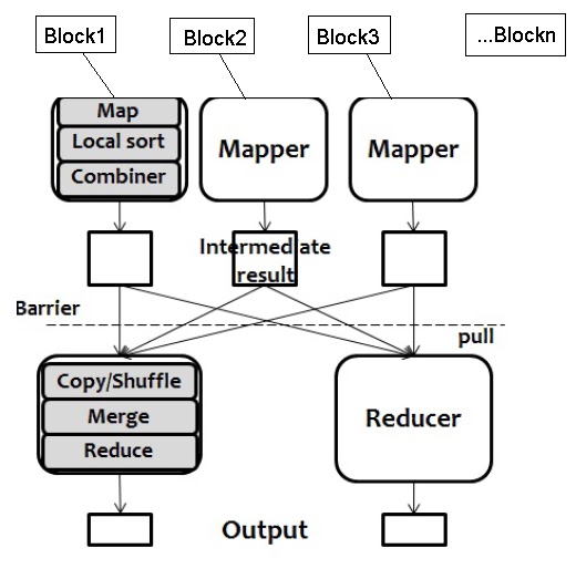
MapReduce Architecture

It consists of two phases:Map and Reduce

 

MapReduce: The Mapper
When the map function starts producing output, it is not simply written to disk. The process is more involved, and takes advantage of buffering writes in memory and doing some presorting for efficiency reasons.Each map task has a circular memory buffer that it writes the output to. The buffer is 100 MB by default, it can change based on the size.When the contents of the buffer reaches a certain threshold size 80%,a background thread will start to spill the contents to disk,during this time, the map will block until the spill is complete.

 

Before it writes to disk,the data is partitions corresponding to the reducers.Each partition,sort by key, and if there is a combiner function,it is run on the output of the sort.so there is less data to write to local disk and to transfer to the reducer.
The Mapper reads data in the form of key/value pairs and It outputs zero or more key/value pairs.
MapReduce Flow-The Mapper
Each of the portions (RecordReader, Mapper, Partitioner,Reducer, etc.)

 

MapReduce: The Reducer
The map output file is sitting on the local disk of the machine.The reduce task needs the map output for its particular partition from several map tasks across the
cluster. The map tasks may finish at different times, so the reduce task starts copying their outputs as soon as each completes. This is known as the copy phase of the reduce task,by default 5 threads can copy,this we can change by property.
When all the map outputs have been copied, the reduce task moves into the sort phase.For example, if there were 50 map outputs, and the merge factor was 10.then there would be 5 rounds. Each round would merge 10 files into one, so at the end there would be five intermediate files.final round that merges these five files into a single sorted file and move to the reduce phase.The output of this phase is written directly to the output filesystem, typically HDFS.

 

MapReduce Architecture

 

After the Map phase is over, all the intermediate values for a given intermediate key are combined together into a list.This list is given to a Reducer

• There may be a single Reducer, or multiple Reducers
• This is specified as part of the job configuration
• All values associated with a particular intermediate key are guaranteed to go to the same Reducer
• The intermediate keys, and their value lists, are passed to the Reducer in sorted key order
• This step is known as the ‘shuffle and sort’

 

The Reducer outputs zero or more final key/value pairs

• These are written to HDFS
• In practice, the Reducer usually emits a single key/value pair for each input key

The MapReduce Flow: Reducers to Outputs.

• Each of the portions (Reducer,RecordWriter,output file)

What is MapReduce

MapReduce published in 2004 by google.Hadoop can run MapReduce programs written in various languages like Java, Ruby, Python, and C++.It consists of two phases: Map and then Reduce and two stage known as the shuffle and sort.Map tasks work on relatively small portions of data – typically a single HDFS block.MapReduce is a method for distributing a task across multiple nodes.Features of MapReduce is to automatic parallelization and distribution.

Shuffle and Sort
MapReduce makes the guarantee that the input to every reducer is sorted by key.It is known as the shuffle.
Counters
Counters are a useful channel for gathering statistics about the job: for quality control or for application level-statistics.
Secondary Sort
The MapReduce framework sorts the records by key before they reach the reducers.

HDFS Architecture

Namenodes(Master Node) - Its keep the address of the file.
Datanode(Slave Node) -   Its keep the actual data.

HDFS has a master and slave node architecture.An HDFS cluster consists of a single Namenode,secondary Namenode and Datanodes.A master node that manages the file system namespace and regulates access to files by clients.Without NameNode, there is no way to access the files in the HDFS cluster.Slave node manages Datanode and Datanode keep the actual data.It allows user data to be stored in files. Internally, a file is split into one or more blocks and these blocks are stored in a set of Datanodes.The Datanodes are responsible for serving read and write requests from the file system’s clients. The Datanodes also perform block creation, deletion, and replication upon instruction from the Namenode.

Data Replication
HDFS stores each file as a sequence of blocks, all blocks in a file except the last block are the same size. The blocks of a file are replicated for fault tolerance. The block size and replication factor are configurable per file. An application can specify the number of replicas of a file. The replication factor can be specified
at file creation time and can be changed later. Files in HDFS are write-once and have strictly one writer at any time. The Namenode makes all decisions regarding replication of blocks. It periodically receives a Heartbeat and a Blockreport from each of the Datanodes in the cluster. Receipt of a Heartbeat implies that the Datanode is functioning properly. A Blockreport contains a list of all blocks on a Datanode.

Secondary NameNode
The secondary NameNode merges the file system image and the edits log files periodically and keeps edits log size within a limit. It is usually run on a different machine than the primary NameNode since its memory requirements are on the same order as the primary NameNode. The secondary NameNode is started by bin/start-dfs.sh on the nodes specified in conf/masters file. The secondary NameNode stores the latest checkpoint in a directory which is structured the same way as the primary NameNode's directory. So that the check pointed image is always ready to be read by the primary NameNode if necessary.

What is HDFS

HDFS, the Hadoop Distributed File System, is responsible for storing data on the cluster.
HDFS is a filesystem written in Java,based on Google’s GFS and Sits on top of a native filesystem Such as ext3, ext4 or xfs.
HDFS is a filesystem designed for storing very large files and running on clusters of commodity hardware.
Data is split into blocks and distributed across multiple nodes in the cluster

• Each block is typically 64MB or 128MB in size
• Each block is replicated multiple times
• Default is to replicate each block three times
• Replicas are stored on different nodes

Files in HDFS
Files in HDFS are ‘write once’ - No random writes to files are allowed
Files in HDFS are broken into block-sized chunks,which are stored as independent units.

When data is loaded into the system, it is split into ‘blocks’ - Typically 64MB or 128MB.
A good split size tends to be the size of an HDFS block, 64 MB by default, although this can be changed for the cluster.In file system there are three types of permission: the read permission (r), the write permission (w),and the execute permission (x).

Namenode
Without the metadata on the NameNode, there is no way to access the files in the HDFS cluster.
When a client application wants to read a file:

• It communicates with the NameNode to determine which blocks make up the file, and which DataNodes those blocks reside on
• It then communicates directly with the DataNodes to read the data.

What is Bigdata? A statistical analysis of ONE MINUTE internet search.

• Google receives over 2,000,000 search queries.
• Facebook receive 34,722 “likes”.
• Consumers spend $ 272,070 on web shopping.
• Apple receives 47,000 Apps downloads.
• 370,00 minutes of calls on Skype,
• 98,000 posts on tweets,
• 20,000 posts on Tumblr,
• 13,000 hours of music streaming on Pandora,
• 12,000 new ads on Craigslist,
• 6,600 pictures uploaded to Flickr,
• 1,500 new blog posts,
• 600 new YouTube videos.